Original Paper: Curiosity-driven Exploration by Self-supervised Prediction
Introduction
Problem Statement: In real-world scenarios, extrinsic rewards are often sparse or absent, necessitating the use of intrinsic rewards.
Key Contributions:
- Curiosity is defined as the error in an agent’s ability to predict the consequences of its actions in a visual feature space learned by a self-supervised inverse dynamics model. This definition is suitable for high-dimensional continuous state spaces like images, bypassing the challenge of directly predicting pixels while ignoring environmental factors irrelevant to the agent.
- The proposed method is evaluated in two environments: VizDoom and Super Mario Bros.
- Three primary scenarios are investigated:
- Sparse extrinsic rewards, where curiosity enables the agent to achieve goals with fewer interactions;
- Exploration with no extrinsic rewards, where curiosity drives more efficient exploration;
- Generalization to unseen scenarios (e.g., new levels of the same game), where knowledge from prior experience accelerates exploration compared to starting from scratch.
Method
The framework consists of two networks: a policy network and the ICM (Intrinsic Curiosity Module).
Policy Network Training
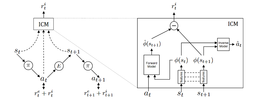
The policy network $\theta_{P}$ is trained as shown in the left figure. At state $s_{t}$, the agent samples an action $a_{t}$ from the current policy $\pi$ and interacts with the environment to transition to state $s_{t+1}$. The policy $\pi$ is optimized to maximize the sum of the extrinsic reward $r_{t}^{e}$ provided by the environment $E$ and the intrinsic curiosity reward $r_{t}^{i}$ generated by ICM:
$$\max_{\theta_{P}}\mathbb{E}_{\pi(s_{t};\theta_{P})}\left[\sum_{t}r_{t}\right]$$ICM Training
The ICM consists of two models: the forward model and the inverse model.
Inverse Model Training
The inverse model first encodes the raw states $s_{t}$ and $s_{t+1}$ into feature vectors $\phi(s_{t})$ and $\phi(s_{t+1})$ using a feature network. It then takes $\phi(s_{t})$ and $\phi(s_{t+1})$ as inputs to predict the action $\hat{a}_{t}$ taken by the agent to transition from $s_{t}$ to $s_{t+1}$. The network parameters $\theta_{I}$ are optimized by minimizing the loss function $L_{I}$:
$$\min_{\theta_{I}}L_{I}(\hat{a}_{t},a_{t})$$Here, $L_{I}$ measures the discrepancy between the predicted and actual actions.
Forward Model Training
The forward model takes $a_{t}$ and $\phi(s_{t})$ as inputs and predicts the feature encoding $\hat{\phi}(s_{t+1})$ of the next state. The network parameters $\theta_{F}$ are optimized by minimizing the loss function $L_{F}$:
$$L_{F}(\phi(s_{t}),\hat{\phi}(s_{t+1}))=\frac{1}{2}\left\|\hat{\phi}(s_{t+1})-\phi(s_{t+1})\right\|_{2}^{2}$$Intrinsic Reward Calculation
The intrinsic reward signal $r_{t}^{i}$ is computed as:
$$r_{t}^{i}=\frac{\eta}{2}\left\|\hat{\phi}(s_{t+1})-\phi(s_{t+1})\right\|_{2}^{2}$$where $\eta>0$ is a scaling factor.
Design Philosophy of ICM
In short, ICM calculates intrinsic rewards using two consecutive states and the action between them, treating state prediction error as curiosity. This explains the need for the forward model, which predicts the next state. But why introduce the inverse model? The authors argue that state information can be divided into three parts:
- Aspects controllable by the agent;
- Aspects uncontrollable but affecting the agent;
- Aspects neither controllable nor affecting the agent (e.g., background elements like swaying leaves).
A good representation should include the first two while excluding the third. The inverse model is designed to predict actions, helping the model discern which state features are influenced by actions, thereby yielding a more meaningful state representation.
Training Details
- Input RGB images are converted to grayscale and resized to 42×42. The state $s_{t}$ is a stack of the current frame and the three preceding frames.
- In VizDoom, actions are sampled every four frames during training and every frame during testing. In Mario, actions are sampled every six frames during training.
- The policy uses A3C, implemented as a convolutional network with four layers, LSTM, and fully connected layers.
- The inverse model in ICM uses four convolutional layers to map the input state $s_{t}$ to the feature vector $\phi(s_{t})$, followed by fully connected layers. The forward model is a fully connected network.
- The overall training objective combines the losses of all three networks: